MM Algorithm

In this article I'll be discussing the Minorise Maximisation (MM) algorithm and working through a few examples. Before I discuss this algorithm I must discuss some background theory.

Background Theory

First Order Optimisation

To find maximums and minimums of a function $f(x)$ we take the derivative, set it equal to 0 and solve for x. In the multivariable case we take the gradient $\nabla f(\tilde{x})$, set it equal to the zero vector and solve for each of the $x_i$ in the $i_{th}$ row of the gradient vector. Note that for the multivariable case we can also get saddle points.

Lagrange Multipliers

For constrained optimisation we want to optimise a function $f(\tilde{x})$ subject to an equality constraint $g(\tilde{x})=0$. To do this we form the Lagrangian $L(\tilde{x},\lambda)=f(\tilde{x})+\lambda g(\tilde{x})$, where $\lambda$ is known as the Lagrange multiplier. We then take the derivatives with respect to each of the $x_i$ and $\lambda$ and solve the resulting system of equations to determine the value of $\lambda$ and then the stationary points.

Convexity and Jensen's Inequality

A function is convex if for all $0\leq t\leq 1$ and all $\tilde{x}_1$, $\tilde{x}_2$ in the domain of the function we have: $$f(t\tilde{x}_1+(1-t)\tilde{x}_2)\leq tf(\tilde{x}_1)+(1-t)f(\tilde{x}_2)$$ To gain some intuition for this inequality note that the right hand side is the line between $(\tilde{x}_1,f(\tilde{x}_1))$ and $(\tilde{x}_2,f(\tilde{x}_2))$ and the left hand side is the function evaluated on the line between $\tilde{x}_1$ and $\tilde{x}_2$. This basically states that the line between any two points in the domain of the function must lie above or on the surface of the function.

Jensen's inequality generalises the above inequality and states that for a real convex function $f$, $x_1,...,x_n$ in the domain of $f$ and positive weights $w_1,...,w_n$ we have: $$f\left(\frac{\sum_{i=1}^{n}w_ix_i}{\sum_{i=1}^{n}w_i}\right)\leq\frac{\sum_{i=1}^{n}w_if(x_i)}{\sum_{i=1}^{n}w_i}$$

Maximum Likelihood Estimation (MLE)

For MLE we want to estimate the parameters of a probability distribution $P(x;\theta)$ given an i.i.d (independent and identically distributed) sample of data from it, $X=(x_1,...,x_n)^T$. We can do this through finding the maximum of the log likelihood function or minimum of the negative log likelihood function. $$\arg\max_{\theta}\log L(X;\theta)=\arg\max_{\theta}\log\left(\prod_{i=1}^{n}P(x_i;\theta)\right)$$ $$\arg\min_{\theta}-\log L(X;\theta)=\arg\min_{\theta}-\log\left(\prod_{i=1}^{n}P(x_i;\theta)\right)$$ Note that the $\log$ is the natural logarithm, we take it as it is often easier to work with and it is an equivalent optimisation problem. We also take the product of probability distributions evaluated at the observations as this is their joint density via the assumption that the observations are independent and identically distributed.

Posterior Probabilities

A latent variable $z_i$ gives information about which component of a mixture model that $x_i$ is drawn from and it equals 1 if $x_i$ is from component j of the mixture model and 0 if it isn't. This latent variable is unobservable and thus we need some way to estimate it. We can accomplish this by working out the probability via Baye's theorem that a given obseration $x_i$ was drawn from the $j_{th}$ component of the mixture model. \begin{align*} p_{j}(z_{i})&=p(z_{i}=1|x_i)\\ &=\frac{p(z_{i}=1)p(x_i|z_{i}=1)}{p(x_i)}\\ &=\frac{\pi_jP(x_i;\theta_{j})}{\sum_{h=1}^{g}\pi_{h}P(x_i;\theta_{h})} \end{align*} Here $p(z_{i}=1)=\pi_j$ as this probability is just the proportions of the mixture model, $ p(x_i|z_{i}=1)=P(x_i;\theta_{j})$, i.e. the probability distribution from the $j_{th}$ component of the mixture model as we are given which component that our observation is from and finally we have $p(x_i)=\sum_{h=1}^{g}\pi_{h}P(x_i;\theta_{h})$ which is just the mixture distribution.

MM Algorithm and Conditions

The MM algorithm can be used for both minimisation and maximisation problems. It accomplishes this through iterativly coming up with better estimates for the optimal value of an objective function, $f(\tilde{x})$. This iterative method is derived by carefully constructing a "surrogate" function $g(\tilde{x}|\tilde{x}_m)$. This surrogate function must satisfy two conditions which for the maximisation version of the algorithm are:

Condition 1

$g(\tilde{x}|\tilde{x}_m)\leq f(\tilde{x})$

Condition 2

$g(\tilde{x}_m|\tilde{x}_m)=f(\tilde{x}_m)$

Note that for the minimisation version of the algorithm we reverse the inequality in condition 1. We then get the algorithm for the updated value at each step of the algorithm via:

$\tilde{x}_{m+1}=\arg\max_{\tilde{x}}g(\tilde{x}|\tilde{x}_m)$

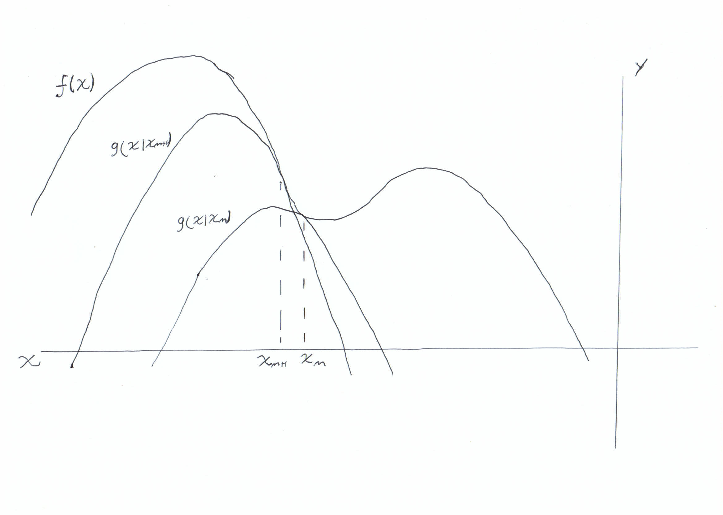
In the above graph we can see intuitively how the algorithm works. The surrogate function is always less than or equal to the objective function (condition 1). There is a point $x_m$ known as the anchor point, which is the single point at which the surrogate function touches the objective function (condition 2). We then update by taking the maximum of the surrogate function and using it as the new anchior point $x_{m+1}$ and this updated surrogate function also adheres to the two conditions.

These conditions along with the algorithm for getting the updated values then yields the following chain of inequalities:

$f(\tilde{x}_{m+1})\geq g(\tilde{x}_{m+1}|\tilde{x}_m)\geq g(\tilde{x}_m|\tilde{x}_m)=f(\tilde{x}_m)$

Which guarentees convergence as the update always increases the value of the objective function (decreases for minimisation (reverse inequalities)).

Common Inequalites Used in Derivation

In order to construct a surrogate function which adheres to the conditions of the algorithm a few common inequalities are generally used:

Cauchy-Schwarz

$|\langle u,v\rangle|\leq\langle u,u\rangle\cdot\langle v,v\rangle$

AM-GM

$\sqrt[n]{\prod_{i=1}^{n}x_i}\leq\frac{\sum_{i=1}^{n}x_i}{n}, \;\;\;\;\;x_1,...,x_n\geq0$

Jensen's

$\phi\left(\frac{\sum_{i=1}^{n}a_ix_i}{\sum_{i=1}^{n}a_i}\right)\leq \frac{\sum_{i=1}^{n}a_i\phi(x_i)}{\sum_{i=1}^{n}a_i}$,$\;\;\;\;\; \phi$ is a convex function and $a_1,...,a_n\geq0$. Note that $x_1,...,x_n$ are in the domain of $\phi$

Quadratic Upper Bound Principle

For minimisation algorithms we can use the quadratic upper bound principle to construct the surrogate function. This is accomplished via using the second order Taylor expansion around $x_m$: $f(x)=f(x_m)+f'(x_m)(x-x_m)+\frac{1}{2}f''(z)(x-x_m)^2$, $z\in[x,x_m]$ If the second derivative of $f(x)$ is bounded above by a positive constant $B$, then $g(x|x_m)=f(x_m)+f'(x_m)(x-x_m)+\frac{1}{2}B(x-x_m)^2$ majorises $f(x)$ with anchor point $x_m$. Note that for the multi variable case $B$ is a positive definite matrix such that $B-H_f$ is positive semidefinite where $H_f$ is the Hessian of the objective function.

Cosine Minimisation Algorithm

For our first example we will start simple by deriving an MM algorithm for finding the minimum of the cosine function. We will accomplish this using the quadratic upper bound principle. Firstly the second order Taylor expansion of cosine is: $\cos(x_2)=\cos(x_1)-\sin(x_1)(x_2-x_1)-\frac{1}{2}\cos(z)(x_2-x_1)^2$ for some $z\in[x_1,x_2]$. Given that the second derivative $-\cos(z)\leq1$, via quadratic upper bound principle we get the surrogate function $g(x_2|x_1)=\cos(x_1)-\sin(x_1)(x_2-x_1)+\frac{1}{2}(x_2-x_1)^2$. Now we maximise the surrogate function by taking the derivative wrt $x_2$ and setting it equal to 0, yielding $\frac{d}{dx_2}g(x_2|x_1)=-\sin(x_1)-x_1+x_2=0\iff x_2=x_1+\sin(x_1)$. Which gives the update $x_{m+1}=x_m+\sin(x_m)$. This can then be implemented in python giving the following code block.


import numpy as np

def MMcos(x,maxiter):
    updates = [x]
    for i in range(maxiter):
        updates.append(updates[i] + np.sin(updates[i]))
    cosine = np.cos(np.array(updates))
    return updates, cosine

Running the code we get the following results:

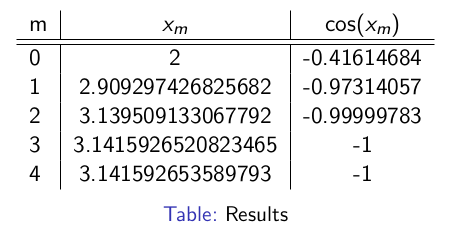
The minimum of cosine is -1 so our algorithm has converged to the correct value.

Poisson Mixture Model

First recall that the Poisson distribution is:

$p(x;\phi)=\frac{\phi^x\exp{(-\phi)}}{x!}$, where $\phi$ is a rate parameter.

We also have the Poisson Mixture Distribution:

$P(x;\tilde{\pi},\tilde{\phi})=\sum_{i=1}^{g}\pi_{i}p(x;\phi_i)$, $\pi_i\in[0,1]$, $\sum_{i=1}^{g}\pi_i=1$.

which we will attempt to learn its parameters from data through MLE via the MM algorithm. The data we are given is a collection of observations $Y=(x_1,...,x_n)$ drawn from the Poisson mixture distribution and corresponding unobserved latent variables $Z=(z_1,...,z_n)$ giving the component of the mixture model that $x_i$ is drawn from, where $z_i\sim$Mult$(\pi_1,...,\pi_g)$. From this we get the joint density for a single component as:

$p_j(x_i,z_i)=p_j(x_i|z_i)p_j(z_i)$

Plugging the joint densities into the PMM the negative log likelihood function can be constructed as follows:

$\begin{align*} Q(x;\tilde{\pi},\tilde{\phi})&=-log\left(\prod_{i=1}^{n}\left(\sum_{j=1}^{g}p_j(x_i,z_i)\right)\right)\\ &=-\sum_{i=1}^{n}\log\left(\sum_{j=1}^{g}p_j(z_i)p_j(x_i|z_i)\right)\\ &=-\sum_{i=1}^{n}\log\left(\sum_{j=1}^{g}\tau_{j}^{(m)}(x_i)\pi_{j}p(x_i;\phi_j)\right) \end{align*}$

Where $p_j(z_i)=\tau_{j}^{(m)}(x_i)=\frac{\pi_j^{(m)}p(x_i;\phi_j)}{\sum_{h=1}^{g}\pi_h^{(m)}p(x_i;\phi_h)}$ (these are the posterior probabilities) and $p_j(x_i|z_i)=\pi_jp(x_i|\phi_j)$.

We first consider the sum for just one of the observations $x_i$. The sum inside the logarithm prevents there being an analytical solution so we can construct an MM algorithm to find the maximum likelihood estimates. In this case we will apply Jensen's inequality as $-\log$ is convex. Note that $\sum_{j=1}^{g}\tau_{j}^{(m)}(x_i)=1$.

$\begin{align*} -\log\left(\frac{\sum_{j=1}^{g}\tau_{j}^{(m)}(x_i)\pi_{j}p(x;\phi_j)}{\sum_{j=1}^{g}\tau_{j}^{(m)}(x_i)}\right)&\leq-\frac{\sum_{j=1}^{g}\tau_{j}^{(m)}(x_i)\log(\pi_j p(x;\phi_j))}{\sum_{j=1}^{g}\tau_{j}^{(m)}(x_i)}\\ &=-\sum_{j=1}^{g}\tau_{j}^{(m)}(x_i)\log(\pi_{j}p(x;\phi_j))\\ \end{align*}$

We now see that we can majorise our loss function via:

$\begin{align*} g_i(\theta|\theta^{(m)})&=-\sum_{j=1}^{g}\tau_{j}^{(m)}(x_i)\log(\pi_{j}p(x;\phi_j))\\ &=-\sum_{j=1}^{g}\tau_{j}^{(m)}(x_i)\log(\pi_j)-\sum_{j=1}^{g}\tau_{j}^{(m)}(x_i)(x_i\log(\phi_j)-\phi_j-\log(x_i!))\\ \end{align*}$

Here we have that $\theta=(\tilde{\pi},\tilde{\phi})$. As we are learning the parameters of the model from n observations the final majoriser is $G(\theta|\theta^{(m)})=\sum_{i=1}^{n}g_i(\theta|\theta^{(m)})$. We also see that our optimisation is constrained by $\sum_{j=1}^{g}\pi_j=1$, so we consider the Lagrangian function $L(\theta|\theta^{(m)})=G(\theta|\theta^{(m)})+\lambda\left(\sum_{j=1}^{g}\pi_j-1\right)$

Taking the gradients we get:

$\begin{align*} \nabla_{\pi_j}L(\theta|\theta^{(m)})&=-\frac{1}{\pi_j}\sum_{i=1}^{n}\tau_{j}^{(m)}(x_i)+\lambda\\ \nabla_{\phi_j}L(\theta|\theta^{(m)})&=-\frac{1}{\phi_j}\sum_{i=1}^{n}\tau_{j}^{(m)}(x_i)x_i+\sum_{i=1}^{n}\tau_{j}^{(m)}(x_i)\\ \nabla_{\lambda}L(\theta|\theta^{(m)})&=\sum_{j=1}^{g}\pi_j-1\\ \end{align*}$

Now setting $\nabla_{\phi_j}L(\theta|\theta^{(m)})=0$ and solving for $\phi_j$ gives the update: $$\phi_j^{(m+1)}=\frac{\sum_{i=1}^{n}\tau_{j}^{(m)}(x_i)x_i}{\sum_{i=1}^{n}\tau_{j}^{(m)}(x_i)}$$

and setting $\nabla_{\pi_j}L(\theta|\theta^{(m)})=0$ and solving for $\pi_j$ we get the update: $$\pi_j^{(m+1)}=\frac{\sum_{i=1}^{n}\tau_{j}^{(m)}(x_i)}{\lambda}$$

Now to find $\lambda$ we set $\nabla_{\lambda}L(\theta|\theta^{(m)})=0$, rearrange and substitute in our update for $\pi_j$.

$\begin{align*} \sum_{j=1}^{g}\pi_j&=1\\ &=\sum_{j=1}^{g}\frac{\sum_{i=1}^{n}\tau_{j}^{(m)}(x_i)}{\lambda}\\ \iff \lambda&=\sum_{j=1}^{g}\sum_{i=1}^{n}\tau_{j}^{(m)}(x_i)\\ &=\sum_{i=1}^{n}1\\ &=n \end{align*}$

Plugging $\lambda$ into our update for $\pi_j$ yields: $$\pi_j^{(m+1)}=\frac{\sum_{i=1}^{n}\tau_{j}^{(m)}(x_i)}{n}$$

Using these updates we can now code up an algorithm for MLE of the Poisson mixture model. The code is a little more involved than the cosine example so I won't cover it here but it can be found here. The estimates yielded from running the algorithm give the following model.

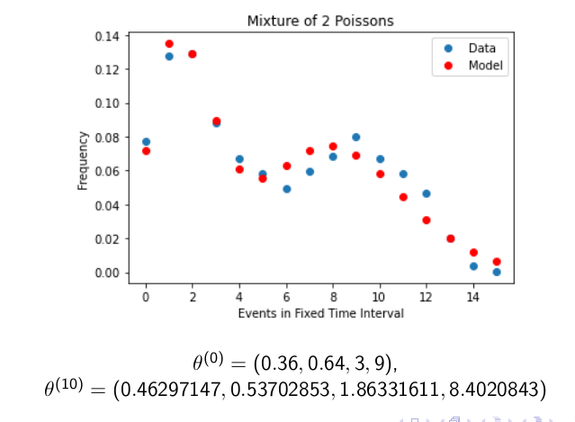
We can see that this approximates the distribution of the data fairly well, indicating that our algorithm was successful. We don't get an exact match as the algorithm has likely converged to a local maximum and not a global maximum. One final note here is that our update yields the same update that we would get from the Expectation Maximisation algorithm (EM) and this is because the EM algorithm is a special case of the MM algorithm.

If you're interested in learning more about this algorithm a good resource is "MM Optimization Algorithms" by Kenneth Lange.