Exploiting Geometry

In this article I'm going to cover one of my favourite proofs I came up with during my undergraduate studies.

For this article I'm going to assume some basic knowledge of statistics, linear algebra and calculus, however those without this knowledge will still be able to appreciate the outline of the proof as it relies heavily on a basic theorem of geometry.

A common task of machine learning is classification, i.e. given some data what class does it belong to. For example we may be given an image of a cat and want an algorithm to classify that image as a cat. Here we will be looking at linear discriminant analysis (LDA), an early classification method developed by Ronald Fischer that produces linear boundaries between classes (e.g. in two dimensions the data will be seperated by lines, in three dimensions planes, and so on and so forth).

LDA assumes that the data in each class follows a multivariable normal distribution with parameters \(\hat{\pi}_j,\hat{\mu}_j\) and \(\hat{\Sigma}\), which is the proportion, mean and covariance matrix of the \(j_{th}\) class respectively (LDA assumes that the covariance matrix is the same for each class). We can estimate the first two parameters via the proportion of data given to belong to class \(j\) and the mean of the data. The common covariance matrix can be estimated by removing the relevant class sample mean from each observation, pooling all the observations and then using the unbiased sample covariance matrix. LDA produces the linear boundaries via the points at which the probabilities of a data point \(x\) belonging to a class \(j\) and a class \(l\) are equal. Using this fact we can derive the discriminant function to decide whether or not \(x\) belongs to \(j\) or \(l\). Note below that the probabilities are given by plugging \(x\) into the multivariable normal distribution for a given class and setting them to be equal (note that p is the dimension of the data).

\begin{align*} \frac{\hat{\pi_j}}{(2\pi)^{p/2}|\hat{\Sigma}|^{1/2}}e^{-\frac{1}{2}(x-\hat{\mu}_j)^T\hat{\Sigma}^{-1}(x-\hat{\mu}_j)}&=\frac{\hat{\pi_l}}{(2\pi)^{p/2}|\hat{\Sigma}|^{1/2}}e^{-\frac{1}{2}(x-\hat{\mu}_l)^T\hat{\Sigma}^{-1}(x-\hat{\mu}_l)}\\ \iff \log\frac{\hat{\pi}_j}{\hat{\pi}_l}&=\frac{1}{2}((x-\hat{\mu}_j)^T\hat{\Sigma}^{-1}(x-\hat{\mu}_j)-\\ &\qquad(x-\hat{\mu}_l)^T\hat{\Sigma}^{-1}(x-\hat{\mu}_l))\\ &=\frac{1}{2}(x^T\hat{\Sigma}^{-1}x-x^T\hat{\Sigma}^{-1}\hat{\mu}_j-\hat{\mu}_j^T\hat{\Sigma}^{-1}x\\ &+\hat{\mu}_j^T\hat{\Sigma}^{-1}\hat{\mu_j}-(x^T\hat{\Sigma}^{-1}x-x^T\hat{\Sigma}^{-1}\hat{\mu}_l\\ &-\hat{\mu}_l^T\hat{\Sigma}^{-1}x+\hat{\mu}_l^T\hat{\Sigma}^{-1}\hat{\mu_l}))\\ \end{align*}

We now notice that the \(x^T\hat{\Sigma}^{-1}x\) terms cancel and that as \(\hat{\Sigma}^{-1}\) is a symmetric matrix we have \(a^T\Sigma^{-1}b=b^T\Sigma^{-1}a\) for \(a,b\in\mathbb{R}^p\). Hence we can now rearrange the equation to:

\begin{align*} &x^T\hat{\Sigma}^{-1}(\hat{\mu}_l-\hat{\mu}_j)=\log\frac{\hat{\pi}_j}{\hat{\pi}_l}+\frac{1}{2}(\hat{\mu}_j^T\hat{\Sigma}^{-1}\hat{\mu}_j-\hat{\mu}_l^T\hat{\Sigma}^{-1}\hat{\mu}_l)\\ \end{align*}

Now setting \(\beta=\hat{\Sigma}^{-1}(\hat{\mu}_l-\hat{\mu}_j)\) and \(\alpha=\log\frac{\hat{\pi}_j}{\hat{\pi}_l}+\frac{1}{2}(\hat{\mu}_j^T\hat{\Sigma}^{-1}\hat{\mu}_j-\hat{\mu}_l^T\hat{\Sigma}^{-1}\hat{\mu}_l)=\log\frac{\hat{\pi}_j}{\hat{\pi}_l}+\frac{1}{2}(\hat{\mu}_l+\hat{\mu}_j)^T\hat{\Sigma}^{-1}(\hat{\mu}_l-\hat{\mu}_j)\) we get the discriminant boundary equation, \(\alpha+x^T\beta=0\). Hence the descriminant function to decide between the \(j_{th}\) and \(l_{th}\) classes is:

\begin{align*} \eta(x)=\begin{cases}j,& \text{ if } \alpha+x^T\beta\geq0\\ l,& \text{ if } \alpha+x^T\beta<0\end{cases} \end{align*}

If we have more than two classes there will be a discriminant function for each pair of classes and the final predicted class is chosen based on all pairwise comparisons. Now that we understand linear discriminant analysis we can state the result we want to prove.

Theorem: For linear discriminant analysis in two dimensions with three classes with known means and common covariance matrix \(\Sigma\) the decision boundaries between pairs of classes intersect a single point under most conditions.

Instead of brute forcing the calculation of the point of intersection we can rely upon a theorem from geometry (*note here that a perpendicular bisector is the line that intersects another line at a right angle).

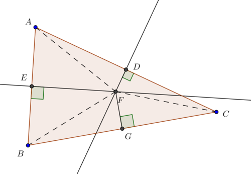
Theorem: Let \(\triangle ABC\) be a triangle. Then the perpendicular bisectors of AB, BC and AC at their respective midpoints all intersect at the same point.

Proof

Let D be the midpoint between AC and E the midpoint between AE. Take the perpendicular bisector of D and E and call the intersection point F. By definition of perpendicular bisector AE=EB and \(\angle AEF= \angle BEF\) are right angles. As E is the midpoint the length of AE=BE and clearly in both the length EF are equal. This means that \(\triangle AEF=\triangle BEF\) and so AF=BF (This is the triangle side-angle-side equality). Similarly we repeat the above reasoning on AD=DC using the triangles \(\triangle ADF\) and \(\triangle CDF\) to get BF=CF. Now let FG be the angle bisector of \(\angle BFC\). We have \(\angle BFG=\angle CFG\) by construction and from above BF=CF. By the triangle side-angle-side equality we get \(\triangle BFG=\triangle CFG\) implying that BG=CG. Now \(\angle BGF=\angle CGF\) meaning that they are right angles and FG is the perpendicular bisector of BC. Now we have that all three perpendicular bisectors intersect at F.

END PROOF

We can now see how this proof is going to play out. We want to show that the boundaries given by LDA intersect the the mid points between the classes at a right angle. As three points in the plane form a triangle, the theorem we just proved will apply.

So first we find the boundary between each of the three classes by performing LDA on each combination of them (AB, AC and BC). We will also use a variant of LDA known as Fisher's LDA that relaxes the assumptions of LDA by not assuming normality of the data and classes not needing to have the same covariance matrix (no model is imposed on the data but the mean vector and covariance matrix of each class is considered). The main idea of Fisher's LDA is to find a univariate projection of the data for which the ratio of between class variance to within class variance is maximised, hence a hyperplane perpendicular to this line then provides the discriminant boundary. In our case we have one common covariance matrix for each class which we will see makes the problem equivalent to standard LDA.

For Fisher's we wish to maximise the difference between the means, normalised by a measure of the within-class scatter. We define the scatter of class j such that \(x_i\in j \;\;\;(i\in1,...,n)\) as: $$\hat{S}_j^2=\sum_{i=1}^{n}(x_i-\mu_j)^2$$ We define the Fischer linear discriminant as the linear function \(a^Tx\) that maximises the criterion function, \(J(a)\), for any two classes as: $$J(a)=\frac{|\mu_1-\mu_2|^2}{\hat{S}_1^2+\hat{S}_2^2}$$ We now need to describe J(a) in terms of a. First we define a measure of scatter as: $$S_j=\sum_{i=1}^{n}(x_i-\mu_j)(x_i-\mu_j)^T$$ Giving the within class scatter matrix: $$S_1+S_2=S_W$$ The scatter of the projection \(x_i\) can now be exprssed as a function of the scatter matrix: \begin{align*} \hat{S}_j^2&=\sum_{i=1}^{n}(x_i-\mu_j)^2\\ &=\sum_{i=1}^{n}(a^Tx_i-a^T\mu_j)^2)\\ &=\sum_{i=1}^{n}a^T(x_i-\mu_j)(x_i-\mu_j)^Ta\\ &=a^TS_ja\\ \end{align*} And hence: $$\hat{S}_1^2+\hat{S}_2^2=a^TS_wa$$ We can also do this for the difference of means giving: \begin{align*} (\mu_1-\mu_2)^2&=(a^T\mu_1-a^T\mu_2)^2\\ &=a^T(\mu_1-\mu_2)(\mu_1-\mu_2)^Ta\\ &=a^TS_Ba\\ \end{align*} Where \(S_B\) is the between class scatter (note the rank of \(S_B\) is one as it is a product of two vectors). Finally: $$J(a)=\frac{a^TS_Ba}{a^TS_wa}$$ We now want to find the max of J(a) with respect to a by taking the derivative with respect to a and equating to zero: \begin{align*} 0&=\frac{d}{da}J(a)\\ &=\frac{d}{da}\frac{a^TS_Ba}{a^TS_wa}\\ &=a^TS_Wa\frac{d(a^TS_Ba)}{da}-a^TS_Ba\frac{d(a^TS_Wa)}{da}\\ &=(a^TS_Wa)2S_Ba-(a^TS_Ba)2S_Wa\\ \iff 0&=S_Ba-J(a)S_Wa\\ &=S_W^{-1}S_Ba-J(a)a\\ \end{align*} We see that this is a generalised eigenvalue problem given by \(S_W^{-1}S_Ba=J(a)a\) whose solution gives \(a=S_W^{-1}(\mu_1-\mu_2)\) and hence the discriminant function is \(a^Tx=x^TS_W^{-1}(\mu_1-\mu_2)\). The discriminant boundary is then given by \(x^Ta+a_0=0\) (here \(a_0\) determines the position of the hyperplane, we can also set this to certain values and rearrange to get the solution from regular LDA hence we see that in this case LDA and Fisher's LDA are equivalent). We then take the boundary to be placed upon the mid point of each of the two class means in this projected space (\(a_0=a^T\frac{\mu_i+\mu_j}{2}\)). Doing this for each case we can form a triangle whose vertices are \(a^T\mu_i\;\;(i\in A,B,C)\) which has discriminant boundaries intersecting it at the midpoints \(a^T\frac{\mu_i+\mu_j}{2}\;\;(i,j\in A,B,C)\). As we have that the discriminant boundaries intersect at the mid points of a triangle formed by the discriminant functions the geometry theorem we proved earlier applies and we have that each of the three classes discriminant boundaries intersect at a single point. We also see in the description of what we are proving that this intersection occurs under most conditions. The condition in which it doesn't occur is if one or more of the vertices \(a^T\mu_i\;\;(i\in A,B,C)\) is projected onto another discriminant line as this will cause the perpendicular boundary lines to be parallel to each other (this occurs as there is no longer a triangle, instead they just all lie on a single line). Hence we have proved the theorem.

Home