Multilayer Perceptrons

This article is going to be a continuation of the previous one on the perceptron. In this article I will explain how the multilayer perceptron (MLP) works and guide you through an implementation of it in python. The article is split into five distinct sections, network architecture, activation functions, forward propagation, backward propagation and training a network on an example dataset.

Network Architecture

We know from the previous article that to get the output of a single perceptron we take the dot product of the input and the weights, but for the multilayer perceptron we link up multiple perceptrons in a series of layers. To maintain the dot product property we can perform a linear transformation of the input \(x\) via \(Wx+b\), i.e. multiply the input vector to each layer by a weights matrix and add the bias vector to it. What this accomplishes is that each of the layers produces exactly the output of several perceptrons, whose input was the vector produced by the previous layer. As each entry in this vector is the dot product of a row of the matrix with the data plus the bias we see that we have succesfully linked together several perceptrons in a series of layers.

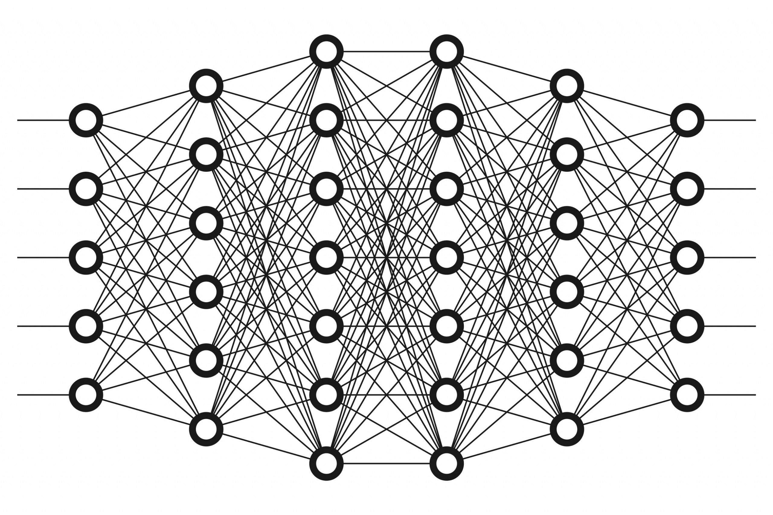
To see this visually we can look at the typical image of a neural network and notice that the connection from the \(j_{th}\) node in layer l to the \(i_{th}\) node in layer l+1 corresponds to the entry \(w_{ij}\) in the matrix \(W_l\). Note here that between each layer we have a weight matrix \(W_l\) and bias vector \(b_l\)

The issue we now face is that we need to set initial weights and biases. A standard practice for this is to draw values from the standard normal distribution \(N(0,1)\), which is implemented below, along with a init method for the MLP class which takes as input two lists. One contains the number of perceptrons in each layer and the other contains strings of the names of the activation function used after each layer.

            def __init__(self, layers, act_fns):
        self.layers = layers
        self.act_fns = act_fns

def initialise(self, w_sig=1):
        W, b = [[]]* len(self.layers), [[]]* len(self.layers)
        for l in range (1, len(self.layers)):
            W[l]= w_sig * np.random.randn(self.layers[l], self.layers[l -1])
            b[l]= w_sig * np.random.randn(self.layers[l], 1)
        
        return W,b

Activation Functions

For MLP's we want to be able to learn more than just linear functions so we require the uasage of functions that aren't linear, dubbed in the literature activation functions. For these functions to work well we require them to have a few properties, mainly that the function is bounded, continous and monotonically increasing. This is due to what is known as the universal approximation theorem which roughly states that with sufficiently many neurons we can approximate any continuous function arbitrarily well. This theorem can sometimes be extended to account for unbounded activation functions that are almost everywhere continous such as ReLU which we will use in this tutorial. Some common activation functions are the sigmoid, tanh and ReLU which are stated below.

\begin{align*} \sigma(x)&=\frac{1}{1+e^{-x}}\\ \text{tanh}(x)&=\frac{e^{2x}-1}{e^{2x}+1}\\ \text{ReLU}(x)&=\max{(0,x)}\\ \end{align*}

We implement ReLU and its derivative in python below.

                    def RELU(z, l, L):
    if l == L: 
        return z, np. ones_like (z)
    else:
        val = np. maximum (0,z)
        J = np.array(z>0, dtype = float )
    return val, J

To utilise these functions in the network we apply them to the output vector of each layer.

Forward Propagation

Now that we understand the structure of the network we require an efficient method for getting from the input vector to the final output prediction. In light of what we have seen above, we see that the network is actually just a composition of linear functions and activation functions. If we denote the linear transformation performed on the input to layer l as \(M_l\) and the activation function applied to it as \(S_l\) we can write the network function \(f(x)\) for an L layered network as \(f(x)=S_L\circ M_L\circ....\circ S_2\circ M_2\circ S_1\circ M_1(x)\). We can now easily implement the network in python using a loop to iterate through each layer.

            def forward(self, x, W, b):
        p = len(self.layers)
        
        a, z, gr= [0]*p, [0]*p, [0]*p
        a[0] = x.reshape(-1,1)
        
        for l in range(1, p):
            z[l] = W[l] @ a[l-1] + b[l]
            a[l], gr[l] = eval(self.act_fns[l])(z[l], l, p-1)
        
        return a, z, gr

Backward Propagation

The only thing thats left to do in this implementation is to have an algorithm to train the network. We first need a way of telling the network how well it did on its prediction. To accomplish this we input the output of the network into a loss function. Before we specify the loss function we denote \(\theta\) as the column vector that contains all the weights and biases of the network (see the appendix for code used in the MLP class that converts the weight matrices and biases vectors into a single vector and vice versa). We can now calculate the loss over n training examples (examples where we are given an input \(x_i\) and output \(y_i\)) via \(\frac{1}{n}\sum_{i=1}^{n}C(y_i, f(x_i|\theta))\). The function \(C(.,.)\) needs to always be positive and thus a common choice is least squares \(C(y_i,f(x_i,\theta))=(y_i-f(x_i,\theta))^2\) which we will use. Another common loss function is cross entropy which is commonly used for classification tasks.

With the loss specified we now need to get good performance from the network. We can approach this as an optimisation problem (minimising the loss on the training data) and thus we use a gradient based method. We need to calculate the gradients with respect to each of the weights and biases in the network. If we denote the output of the linear transformation at layer l as \(z_l\) and \(a_l=S_l(z_l)\) we have:

\begin{align*} \frac{\partial C}{\partial W_l}=\delta_l a^T_{l-1},\;\;\;\frac{\partial C}{\partial b_l}=\delta_l\\ \end{align*}

Where \(\delta_l:=\frac{\partial C}{\partial z_l}\) is computed recursively for \(l=L,...,2\) via:

\begin{align*} \delta_{l-1}=D_{l-1}W^T_l\delta_l,\;\;\;\text{with }\delta_L=\frac{\partial S_L}{\partial z_L}\frac{\partial C}{\partial f}\\ \end{align*}

Here we define \(D_l:=diag(S'(z_{l,1}),...,S'(z_{l,p_l}))\), where \(S'\) denotes the derivative of the activation function. As this is a diagonal matrix its multiplication is componentwise, thus we can redefine the delta calculation to \(\delta_{l-1}=S'(z_{l-1})\bullet W_l^T\delta_l\), where \(\bullet\) is defined as component wise multiplication and \(S'(z_{l-1})\) is the derivative of the output of the activation function of a layer.

def backward(self, W, b, X, y):
        n = len(y)
        L = len(self.layers)-1
        delta = [0] * len(self.layers)
        dC_db, dC_dW = [0] * len(self.layers), [0] * len(self.layers)
        loss = 0
        
        for i in range(n): #looping over training examples
            a, z, gr = self.forward(X[i,:].T, W, b)
            cost , gr_C = SE_loss(y[i], a[L])
            loss += cost/n
            delta [L] = gr[L] @ gr_C
            
            for l in range (L ,0 , -1): # l = L ,... ,1
                dCi_dbl = delta [l]
                dCi_dWl = delta [l] @ a[l-1].T
                # ---- sum up over samples ----
                dC_db [l] = dC_db [l] + dCi_dbl /n
                dC_dW [l] = dC_dW [l] + dCi_dWl /n
                # -----------------------------
                delta[l-1] = gr[l-1] * W[l].T @ delta [l]
        
        return dC_dW , dC_db , loss

This now gives us the method for calculating the gradient of the network which can then be used to train it via gradient decent, i.e. the update at iteration i of training is given by \(x_{i+1}=x_i-\eta \nabla f(x_i)\) (\(\eta\) is the learning rate), which is implemented below.

def train(self, batch_size, num_epochs, lr, W, b, X, y):
        beta = self.list2vec(W,b)
        loss_arr = []
        n = len(X)
        print (" epoch | batch loss")
        print (" ----------------------------")
        for epoch in range (1, num_epochs +1):
            batch_idx = np.random.choice(n, batch_size)
            batch_X = X[batch_idx].reshape(-1 ,1)
            batch_y = y[batch_idx].reshape(-1 ,1)
            dC_dW, dC_db, loss =  self.backward(W, b, batch_X , batch_y)
            d_beta = self.list2vec(dC_dW , dC_db)
            loss_arr.append(loss.flatten()[0])
            if(epoch ==1 or np.mod(epoch ,1000) ==0):
                print (epoch ,": ",loss. flatten () [0])
            beta = beta - lr*d_beta #gradient descent
            W, b = self.vec2list(beta)
        
        dC_dW , dC_db , loss = self.backward(W,b,X,y)
        print (" entire training set loss = ",loss. flatten () [0])
        
        return W, b, loss_arr

Training on an Example Dataset

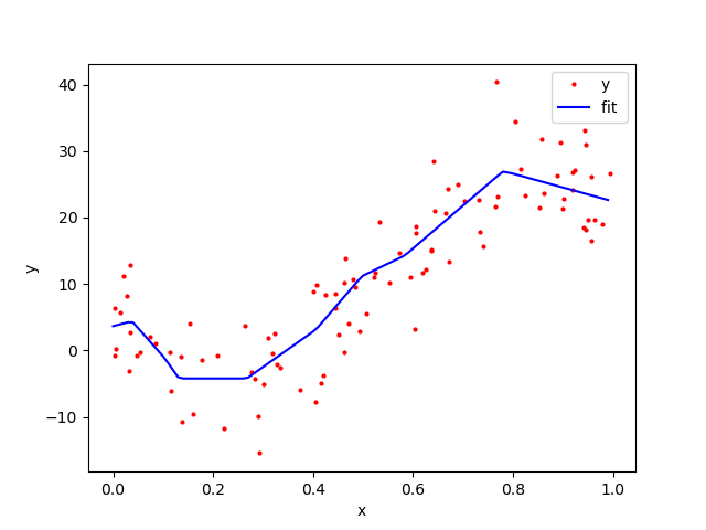
We will now train the network on a dataset given by random values of a polynomial with normally distributed data added to it (you can find the csv file for this data on the github page linked at the bottom). The function we are learning is one that takes a real number as input and gives a real number as output, hence the width of the input and output layers of the network will be 1. For this dataset we can achieve good performance with two hidden layers with width 5 and 7 respectively.

                data = np.genfromtxt('polyreg.csv',delimiter =',') 
X = data[: ,0].reshape( -1 ,1)
y = data[: ,1].reshape( -1 ,1)
layers = [1,5,7,1]
act_fns = ["","RELU","RELU","RELU"]
n = MLP(layers, act_fns)
W, b = n.initialise()
W_f, b_f, loss_arr = n.train(20, 10000, 0.005, W, b, X, y)

The data and the networks predicted function can be seen below. In this we see that the MLP through training has managed to come up with a reasonable approximation to the polynomial function.

Conclusion